 Oxstones Investment Club™
Ever since Harry Markowitz formulated his nobel-prize winning Modern Portfolio Theory, portfolio optimization became a science. MPT’s mean-variance algorithm allows one to calculate the lowest volatility for a given return, or equivalently, the highest return for a given volatility. The model has as inputs the expected returns of the investment universe, the volatilities, and the correlation among each pair of investments within the universe.
The model gave rise to the concepts of beta and the market portfolio and laid the foundations for a rigorous approach to constructing a portfolio that was efficient. But take into consideration the assumptions behind the model and it becomes clear why art comes into play where science leaves off.
Efficient Frontier
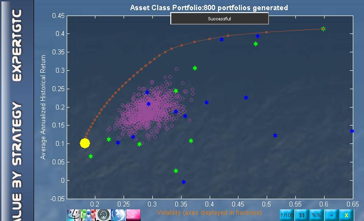 The figure on the left shows the efficient frontier for a selection of securities held by the Harvard Management Corp at the start of 2012. The efficient frontier is the red line on which every portfolio mix has the highest return for a given volatility, and simultaneously, the lowest volatility for a given return. The x-axis measures volatility which is defined by the standard deviation of the expected returns. The expected returns are the averages of historical daily-moving annualized returns. The frontier is unique to the universe of securities which has been used in its calculation. In other words, you can find a unique frontier for every universe of securities you can dream of. In this example, the universe consisted of 22 securities in international stocks and ETFs.
Correlation
The correlations that exist between each pair of 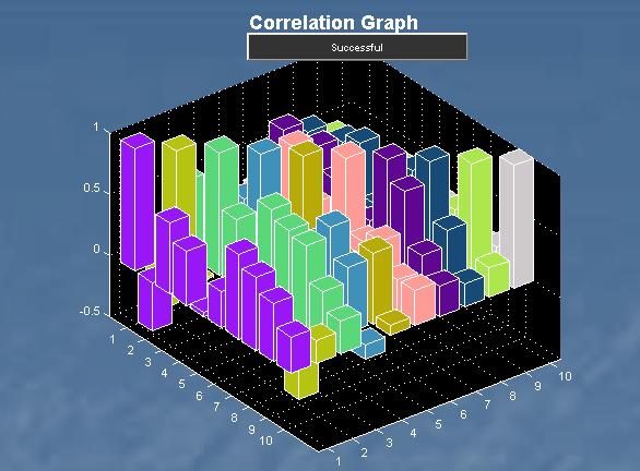 securities in the given universe create the advantage of diversification. This diversification advantage is evidenced by the bulge of the frontier towards the left and upwards direction — the direction of lower volatility and higher return. The bigger the bulge, the more diversification advantage — which is the result of higher correlation among the securities in the negative direction. In fact, as long as correlations are less than perfectly positive, there are some diversification benefits. The figure here shows the correlation among the top 10 holdings of the PowerShares QQQ Trust ETF (QQQ).
Expect the Unexpected
The expected return is the historical average return which is effectively a weighted (by probability) average of past returns. Intuitively, the expected return can also be seen as the return we expect to happen in the future. But why use the past to predict the future? The answer lies in the concept of mean reversion which believes that future returns will oscillate about the historical mean. Reversion to the mean requires that returns obey a probability distribution that is normal. A distribution that is normal has equal probability of occurrence on either side of the mean. So in the long term, the actual return will be near the historical average return. Within this context, using as much historical data as possible to calculate the expected returns makes sense.
The concept can be illustrated as follows:
Say your portfolio returned 4% in year 1, 6% in year 2, and 8% in year 3. The simple average would be 6% which you get by dividing 3 into the sum of 4, 6, and 8. Another way of calculating this average would be to take the simple average at the end of year 2 which is 5% (the sum of 4 and 6 divided by 2) and adding the “impact” that the year 3 return of 8% makes to the average of 5% i.e. 5+(8-5)/3=5+1=6%. The latter way of calculating the average gives you an idea of how the Law of Large Numbers works.
Now, suppose you had 1000 data points (approximately 3 years of daily moving annualized returns), then a big jump or drop at the 1000th data point when divided by the number of data points would have a small “impact” on the mean return (historical average return). For example, if the simple average up to the 999th data point was 5%, then a 40% return in the next data point would only increase the mean return by 0.035% (40-5)/1000).
In practice, we only have so many years of historical data to input into our optimizer to calculate the efficient frontier. But even if we did have a basketfull of historical data as well as a holding period that could extend “forever”, the past may not be altogether helpful in predicting the future if certain conditions do not exist.
Non-normality
Normality is defined by 68% of data being within one standard deviation of the mean, 95% of data being within two standard deviations and 99% being within three standard deviations. It has the standard bell-curve shape that most are familiar with. It has the property of having an equal probability of occurrence on either side of the mean. In other words, it defines randomness.
When distributions are deemed non-normal, they do not follow these specifications. For example, it may be that only 40% of data, rather than 68%, are within one standard deviation of the mean — implying more occurrences nearer the tails than would otherwise occur in a normal distribution. Or it might be that data is not equally distributed on both sides of the mean. For example, there might be 70% on the left and only 30% on the right of the mean– implying non-randomness. The statistical terms of kurtosis and skewness apply respectively. While there are software to estimate such non-normal probability distributions, they sacrifice returns during times of normality and assume that the non-normal distributions that are arrived at are stable ones.
Stationarity
A series of returns might test normal but it could still be non-stationary. Simply put, a time series is stationary if its mean and variance, should they exist, do not change over time. If the mean changes over time, then taking too much past data to calculate the historical average loses information. The information that is lost is the data that reflects recent developments in the market. This information has now been averaged into the long term mean.
So for the mean-variance optimization to do its allocation work, it requires both normality and stationarity as pre-requisites. If returns are normally distributed and their means do not vary with time, they will revert to the mean. If returns are non-normal, the allocations from the mean-variance optimization will be distorted. If the returns are non-stationary, then assuming the optimized allocations remain constant through time may not be true.
A model framework
It has been argued that non-normality may be attributed to the likely existence of mixed normal return distributions. Readers who are interested to do further research can check out Rosenberg, B. (1974). “Extra-Market Components of Covariance in Security Returns.” Journal of Financial and Quantitative Analysis 9(2), 263-273.
The notion is that the “mean and variance” do approximate investors’ expectations at any point of time but that the “returns and variances” vary over time. In this context, a normal return distribution assumption is often appropriate for risk-return estimation at a given point of time.
The research therefore suggests a model framework that makes use of the Markowitz mean-variance algorithm with its normality assumption while acknowledging the fact the varying returns and variances (non-stationarity) should be accounted for during times of rebalancing. For ease of reference, let’s call this approach X3.
To illustrate this, let’s choose a universe where only 1 out of the 8 stocks was not rejected for normality. Statisticians say “rejected for normality” because you cannot say for sure if a distribution is normal, you can only reject the assumption that it is normal at a certain probability level.
The 8 stocks are high volatility stocks selected from the OxStones Stock Picks. The stocks that go into the universe are Archer Daniels Midland Co (ADM), Corning Inc (GLW), Newmont Mining Corp (NEM), Nokia Corp (NOK), Telefonica SA (TEF), Teva Pharmaceuticals Industries Ltd (TEVA), Total SA (TOT), and Yahoo! Inc (YHOO).
Note that the point of this exercise is not to see if the X3 approach yielded the highest returns. Rather, it is to see if the X3 approach out performs the traditional buy & hold for a portfolio that is non-normal and non-stationary in times of boom and bust. Taxes, commissions, and the use of a risk-free proxy are not included in the calculations. The exercise is not offered as a rigorous proof but as an observation on the potential of such an approach.
Conclusion
Buy & hold is a great strategy when you have a portfolio that tests normal and is stationary. Such a portfolio will likely revert to the mean with equal probability from either side of its long-term mean. And the optimization calculations should hold.
A portfolio that tests non-normal will, however, not revert to the mean with equal probability from either side of the mean. Blindly applying an optimizer to a portfolio that tests non-normal will result in distorted allocation weights. On the other hand, maintaining a buy & hold strategy in the face of non-stationarity (even if the portfolio tests normal) will too create sub-optimal results.
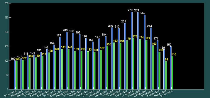
The X3 strategy uses the appropriate formula to calculate expected returns and decide on whether to buy & hold or rebalance depending on whether the assumptions of normality and stationarity hold or have been violated. The figure above shows the performances of 2 portfolios each with a starting value of 100 on 26 January 2006. The blue bars represent the portfolio using the X3 strategy which takes into account non-normality and non-stationarity while the green bars represent a portfolio using a simple buy and hold strategy. The X3 strategy is seen to outperform a simple buy and hold strategy at every review point.
So while the nobel-prize winning mean-variance algorithm is science par excellence, knowing the best way to deploy it, is equally if not more important. This is the art and science of rebalancing.
Tags: correlations, diversification, efficient frontier, expected returns and risks, expertGTC3, investment planning and monitoring system, investment strategies, Markowitz, maurice sakamoto raj, Modern portfolio theory, non-normality, oxstones portfolio analysis, portfolio construction, portfolio volatility, statistical portfolio analysis