 Oxstones Investment Club™
In 1986, Gary P. Brinson, L. Randolph Hood, and Gilbert L. Beebower published a study about the effects of asset allocation of 91 large corporate pension funds measured from 1974 to 1983. The result of the study showed that Asset Allocation (what they called Policy) explained 93.6% of Total Return Variation, Asset Allocation together with timing the market explained 95.3% and Asset Allocation together with stock selection explained 97.8%.
In the study, Investment Policy identified the long-term asset class allocation plan of each fund and was determined by using the funds’ benchmark returns and weights, Policy with timing used actual weights but benchmark returns, Policy with selection used benchmark weights with active returns (actual security returns in excess of benchmark returns).
A Universal Myth
Armed with the findings of this study, some financial advisers were quick to jump on the asset allocation bandwagon. If asset allocation was supposedly the key then stock selection and timing would have little consequence.
But a survey by Nuttall & Nuttall (1998) demonstrates that out of 50 writers who quoted Brinson, only one quoted him correctly. Approximately 37 writers misinterpreted Brinson’s work as an answer to the question, “What percent of total return is explained by asset allocation policy?” and five writers misconstrued the Brinson conclusion as an answer to the question, “What is the impact of choosing one asset allocation over another?”
Ibbotson & Associates called it a universal myth: “From the marketing materials of mutual fund companies and financial planning firms to the mouths of academics and financial representatives, there is a universal misunderstanding of the relationship between asset allocation and performance”.
What the Brinson study describes is the variability (not the return) of the portfolio’s performance over time due to asset allocation i.e. Brinson found that more than 90 percent of the movement of one’s portfolio from quarter to quarter is due to market movement of the asset classes in which the portfolio is invested.
Putting Things In Context
Perhaps what contributed to the myth was the fact that Brinson made a connection between total returns and the variation of returns explained by asset allocation. In the study Brinson did mention that timing deducted 0.66% and stock selection deducted 0.36% from the benchmark annualized total return (not variability) over the 10-year period in his study. And he proceeded to connect this to his statement that asset allocation explained 93.6% of total return variation (not total return), asset allocation with timing explained 95.3% and asset allocation with stock selection explained 97.8%.
In his study Brinson used regression to view the relationship between asset allocation versus actual total return, asset allocation with timing versus actual total return, and asset allocation with stock selection versus actual total return. Based on the presumably linear relationship between the independent and dependent variables, Brinson could get a predicted total return value (the dependent variable) given any value of the independent variables.
The degree of variability of the predicted total return values around the actual average total return divided by the degree of variability of the actual returns around the same actual average total return turned out to be 93.6% for asset allocation, 95.3% for asset allocation with timing, and 97.8% for asset allocation with stock selection. This ratio is termed r-squared in statistical parlance.
Ibbotson did their own study to measure the impact of asset allocation on return level (not return variability). However, rather than using “estimated policy weights and the same asset class benchmarks for all funds, the actual policy weights and asset class benchmarks of the pension funds were used. In each quarter, the policy weights were known in advance of the realized returns”.
The study found that, on average, the policy benchmarks match the actual portfolios, so the ratio is 1.0, or 100 percent. He described it succinctly when he said “Policy benchmarks match the actual portfolios because, if one averages the universe of funds, one gets the index—on average, active management does not provide a return greater than the index”.
Interestingly but not surprisingly, the study also found that about 40 percent of the return difference from one fund to another is explained by policy differences.
Ibbotson concluded in his study that “for the long-term individual investor who maintains a consistent asset allocation and leans towards index funds, asset allocation may very well be the key determinant of his portfolio performance. But for the shorter-term investor who trades more frequently, invests in individual securities, and practices market timing, asset allocation has a lesser impact on returns”.
So notwithstanding the so-called “myth”, both studies seem to allude to the fact that for the long-term investor in indices, active management does not help and at worse, takes away from possible returns.
Diversification versus Optimization
Asset allocation is all about having the right weights placed on each asset class. In the limiting case, if each asset class consisted of just one stock, would the results still hold? No, because the asset class is relatively stable whereas a single stock is volatile.
The asset class is relatively stable because it holds many securities together and is therefore “naively” diversified. I use the word “naively” because there is no formulation behind the weights. They are either equally weighted or weighted by market capitalization.
By stable I am not referring to the statistical concept of stability (unless I otherwise specify) but to returns that revert to their mean. In an index or asset class, returns are assumed to revert to their mean over time. The concept of mean reversion assumes that returns are over the long term normal — in the statistical sense of the word.
Which brings me to another “myth” that the industry got into when optimizers were the rage. With the original “myth” on asset allocation in full swing, some advisers were quick to ask the question that if allocating the right weights to asset classes was important for performance, then feeding security data into an optimizer to come up with the right weights would too yield the ideal portfolio of securities.
Optimizers are tools that calculate efficient portfolios. An efficient portfolio is one which yields the “best” return for a given volatility and simultaneously the least volatility for a given return by calculating the right weights to place on each component of the portfolio. It makes use of the mean-variance algorithm that stems from Modern Portfolio Theory — a theory that won its founder Harry Markowitz a Nobel prize. The theory is taught in all college finance courses and is the cornerstone of almost all financial theory.
The mean-variance algorithm is good theory. But only if the data going into the algorithm are “normal” in the statistical sense. Non-normality can be the result of a non-stationary series. A non-stationary series simply implies that the mean and variance are not constant over time. Non-normality can also be the result of a greater-than-normal number of extreme values in the tail, resulting in what is called a “fat tail”. Such distributions may be stable (in the statistical sense) but have infinite variance (which is effectively variance that is undefined).
Since single securities do not have the benefit of naive diversification like an index does, applying an optimizer to a set of stocks, say, can create an efficient frontier that shifts wildly, unless the stocks themselves are near-normal and likely to revert to their means.
Fat Tails
When the financial world entered an era when rare occurrences, well … occurred, those who thought they knew better cried “fat-tails”. Investors should realize that to take such skewness caused by “fat-tails” into the calculations would mean they have opted for a strategy that underperforms their peers during times of market stability.
The thinner tails of a normal distribution do not mean zero risk.
The normal distribution is a probability distribution and probability is an asymptotic (long-term) concept. In the shorter-term it should not be surprising that a rare occurrence can still occur. While betting on a rare occurrence can apparently make you money if you are the likes of Taleb, abandoning the concept of normality for a fat tail distribution may be just a fanciful way of rationalizing why things occur when they should only rarely occur.
Did you find my statement “rationalizing why things occur when they should only rarely occur” strange? You should.
While the study of fat-tail distributions is an interesting and advanced area of mathematics, using tools that assume normality and adjusting for rare occurrences is a simpler and, dare I say, better approach. It’s simpler because we are not over-fitting historical data with a complicated model in order to predict the future. It’s better because it is a strategy that performs during times of market stability which occurs, by definition, more often than a rare event.
A Method To The Myth
Whatever the actual degree that asset class allocation plays in determining portfolio total return, it is without doubt an important factor. Asset allocation has to do with finding the right weights. An optimizer can find the right weights for inputs assuming these inputs revert to their means some time in the future.
But what if the inputs are not likely to revert to their means, such as in the case of many individual securities?
Drawing from the notion that returns can result from a mix of normal probability distributions, and using an actuarial approach that has been the subject of our research, we will attempt to apply the principle of asset class allocation to asset allocation at the security level by optimizing a portfolio of selected stocks and re-balancing at non-regular intervals of time that have been automatically determined. The portfolio that has been subjected to this process will be called a re-engineered portfolio.
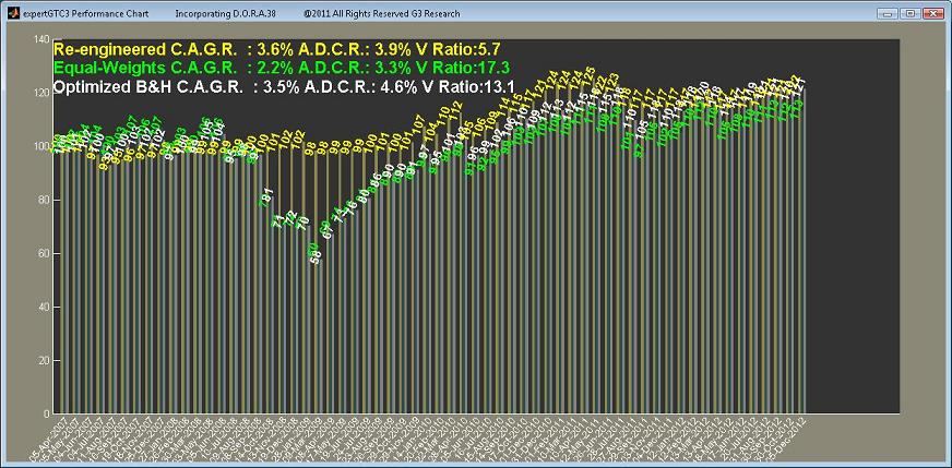
In the illustrations that follow, we use starting portfolio values of $100 so it is easy to get a quick appreciation of their percentage growth. Taxes, commissions, and the use of a risk-free proxy (unless implicitly included as in case 1 below) are not included in the calculations. Price data has been sourced from Yahoo Finance on a dividend-adjusted basis. The results are true-tests, obtained by going back in time to use only the data available as at each review point, calculating the weights, then going forward to compare the performance between the re-engineered (gold), equal-weights (green) and optimized buy & hold (grey) portfolios. The portfolios are assumed to be 100% invested throughout. C.A.G.R. denotes the Compounded Annualized Growth Rate and A.D.C.R. is the mean Annualized Daily Compound Rate. The V Ratio measures the standard deviation of the Annualized Daily Compound Rates divided by the A.D.C.R.
1. Indexes
The universe here consists of Vanguard Total Stock Market ETF (VTI), Vanguard MSCI Emerging Markets ETF (VWO), Vanguard REIT Index ETF (VNQ), and iShares Barclays 1-3 Year Treasury Bond ETF (SHY).
Since the indices are intrinsically “naively” diversified, we would expect the performance of the optimized buy & hold portfolio to be the best performer. The figure shows that the re-engineered portfolio and the optimized buy-and-hold perform very closely. But the re-engineered portfolio avoided the dip in mid-2008 unlike the equal-weights and optimized buy & hold portfolios which fell in tandem.
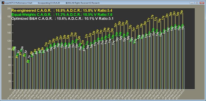
2. Securities for long term holding
The stock universe consists of the following 21 stocks. These are stocks that someone like Warren Buffett might hold (and he has) in his portfolio. They are for the long term and presumably will return to the mean some time along the way. As such, we would expect the optimized buy & hold portfolio to hold its own against the equal-weights portfolio. The figure shows that it indeed has but notice the re-engineered portfolio (gold) still appears to do slightly better than both.
American Express Company(AXP), ConocoPhillips(COP), Costco Wholesale Corp(COST), Exxon Mobil Corp(XOM), General Electric Company(GE), GlaxoSmithKline(GSK), Ingersoll Rand(IR), Johnson & Johnson(JNJ), Kraft Foods Inc(KFT), M&T Bank Corp(MTB), Moody’s Corp(MCO), Procter & Gamble Co(PG), Sanofi American Depositary(SNY), The Bank of NY Mellon Corp(BK), The Coca Cola Company(KO), The Washington Post Company(WPO), Torchmark Corp(TMK), US Bancorp(USB), United Parcel Service(UPS), Wal-Mart Stores Inc(WMT), Wells Fargo & Company(WFC)
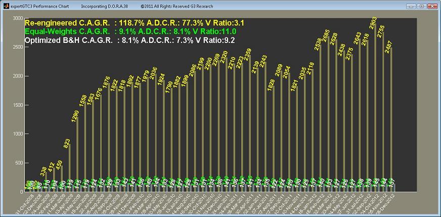
3. Securities for trading
Finally, let’s take a look at a high volatility portfolio consisting of the stocks below, most of which come from the OxStones Investment Club. Since they are high volatility and presumably unstable in the sense that they might not revert to their means, we would expect the optimized buy & hold to not do any better than the equal-weights portfolio over the long term.
As shown in the figure below, this is the case. But what is striking is the fact that the re-engineered portfolio (gold) had a compounded annualized growth rate of almost 119% during this period i.e. any amount invested in the re-engineered portfolio on 31st Oct 2008 would have grown 24.87 times by 8th Dec 2012!
The compounded growth of any portfolio depends on the day it starts and the day it ends so this high performance could be unique to that period. What is important is if the re-engineered portfolio consistently beats the equal weights portfolio.
By doing many runs on different start days with different holding periods, there has not yet been a time when the re-engineered portfolio did not beat the equal-weights portfolio, but needless to say, our research continues.
Stocks in the High-Volatility Model Portfolio (stocks in Italics are sourced from the OxStones Investment Club: Alumina Ltd (AWC), Aluminum Corp Of China Ltd (ACH), Arch Coal (ACI), Archer Daniels Midland Company (ADM), Best Buy Co (BBY), CEMEX, S.A.B. de C.V. (CX), CNH Global NV (CNH), Cameco Corp (CCJ), Central European Dist Corp (CEDC), Central European Media Ent Ltd (CETV), China Life Insurance Co. Ltd (LFC), Coca Cola (KO), Coeur d’Alene Mines Corp (CDE), Corning (GLW), DRDGOLD Ltd (DRD), Fibria Celulose SA (FBR), France Telecom (FTE), GOL Linhas Areas Inteligentes SA (GOL), Harmony Gold Mining Co. Ltd (HMY), Humana Inc (HUM), Impala Platinum Holdings Ltd (IMPUY.PK), Kinross Gold Corp (KGC), McDonald’s Corp (MCD), Net 1 Ueps Technologies (UEPS), Newmont Mining Corp (NEM), Nokia Corp (NOK), Oi SA (OIBR), Potash Corp of Saskatchewan (POT), Owens-Illinois (OI), Petroleo Brazileiro (PBR), Pilgrim’s Pride Corp (PPC), Repsol Ypf SA (REPYY.PK), Telefonica SA (TEF), Teva Pharmaceutical Ind Ltd (TEVA), Total SA (TOT), Universal Corporation (UVV), Veolia Environnement SA (VE), Wal-Mart Stores (WMT), Western Refining Inc. (WNR), Yahoo! (YHOO)
Conclusion
Myths are created when people mis-quote or mis-interpret. This is because language is an imprecise medium when it tries to translate the precision with which mathematics expresses its concepts.
The bottom line, as the studies in this article have shown, is that for the long-term individual investor who maintains a consistent asset class allocation and leans towards index funds, asset class allocation may very well be the key determinant of his portfolio performance. But for the shorter-term investor who trades more frequently, invests in individual securities, and practices market timing, asset class allocation has a lesser impact on returns.
The results from our own tests do not detract from the findings of Brinson or Ibbotson. What we have done is taken the often mis-applied mean-variance optimization algorithm, applied it at the security level, and subjected the portfolio to a unique re-balancing procedure which takes care of the normality assumption.
The procedure automatically selects the right time to re-balance so there is an element of timing. And while stock selection can impact its overall return, the strength of the procedure lies in never under-performing its equal-weighted portfolio benchmark.
Were the re-engineered results just a rare occurrence? Were they a fat-tail event? Is it now possible that for the shorter-term investor who trades frequently, puts the right weights on well-researched individual securities, and practices market timing using a formulaic procedure, to add to and not deduct from total returns based purely on asset class allocation?
There may yet be a method to the myth.
Tags: asset allocation, brinson study, index funds, investment strategies, long term investing, marketing timing, mean-variance in portfolio returns, Modern portfolio theory, optimized portfolios, risk and reward, security selection, short term investor, time horizon and impact from asset allocation, volatility in portfolio returns