 Oxstones Investment Club™
In the first installment of this 3 part message on my blog at expertgtc3.wordpress.com we began with a description of how you should be aware of the risk in any portfolio. I also mentioned that having a strategic portfolio which allocates across different assets or asset classes helps to ensure that you capitalize on movements in assets that do not correlate in a bad way with each other.
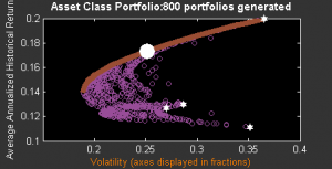
Figure 1
The red line in Figure 1 is the efficient frontier which would be straight if not for the benefits of negative correlation (or more precisely, less than perfectly positive correlation).
To the extent that 2 assets are less than perfectly positively correlated, volatility can be reduced. Obviously, the more non-positively correlated, or even better, negatively correlated the greater the benefit. This benefit arises because the covariance of these 2 assets is reduced the lower the correlation between them. See Figure 2.
Since covariance is a component of total portfolio variance, the lower this value the lower will be the volatility risk of your portfolio.

Figure 2
The calculations are straight forward when there are only 2 assets but increase exponentially in complexity the more assets you have. For example, with just 30 assets there are 1,073,741,793 combinations for you to analyse. Fortunately, computer software is good at doing this kind of thing.
In Part 2 of this series in my blog, I explained why it was dangerous to time the market as in most cases, there is evidence to suggest that the market behaves in a random fashion. Believing that someone can time the market, detect a trend, or do a long term forecast are all akin to trying to drive a car blindfolded while having someone give you instructions looking at the rear-view mirror.
Given these 2 considerations, what would be a better way of constructing your portfolio so that you have a better chance of achieving your life goals?
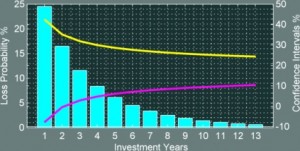
Figure 3
Simply by finding a good set of diversified assets and letting time further diversify away portfolio volatility risk. In Figure 3, the blue bars show reducing probability of negative returns as the funnel (volatility) squeezes in. The funnel is an interval formed by taking volatility bounds on both sides of the historical mean which can be read off the second y-axis on the right hand side of the graph. Notice that the rate of volatility reduction slows down as time passes and this can be seen by the tapering off of the funnel.
How long term allocation works

The figure shows the difference returns (i.e. annual returns minus the average return) for the Dow Jones Industrial Average (blue bars) over the period May 6, 1982 to April 29, 2011 compared against a random distribution with the same mean and standard deviation (red bars)
With long term allocation, we don’t time the market. We believe the market is approximately normal and returns in any one period will gradually move back towards their historical mean in a subsequent period. Note: It’s important how you calculate this historical mean.
The rule of thumb is to re-balance your portfolio to its optimal mix once a year (Note: there is a more precise way of determining the re-balancing interval). In the case of a 2-asset portfolio, when one asset rises, there is an over-allocation of this asset so we sell off some of this asset to bring the allocation back to its original allocation. At the same time, the other asset may fall so there is an under-allocation and we buy more of that asset to bring the portfolio back to its original allocation. This is the act of re-balancing.
If the assets you or your adviser have chosen are nicely diversified and move out of tandem with each other, re-balancing becomes a straight-forward exercise. But the 2 assets may not be perfectly negatively correlated and so there will be situations when they are both on the rise or both on the decline.
Furthermore, asset returns drift (Figure 4) as time goes by.
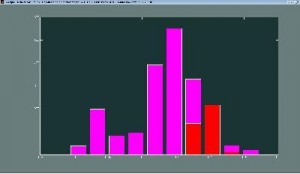
Figure 4
While the accumulation of all these returns drifting through time charts a near normal distribution (the purple bars), the time it takes to return to the historical mean may in certain cases appear to be a trend with no end in sight. This could pose a problem — psychologically, although technically, there are ways to get around this. But more on this in a later article.
Another Consideration
Let’s recap by re-tracing our steps. We have arrived at a portfolio mix that promises us the most return for a given volatility or similarly, the least volatility for a given return. The inputs into this efficient portfolio are the historical mean returns, their volatilities, and most significantly, the correlations among the component assets of this portfolio. Selecting assets that are negatively correlated to each other lowers the portfolio volatility. Seen another way, selecting assets that are negatively correlated allows us to choose a portfolio with a higher return for a volatility level that we can bear.
But lower portfolio volatility does not mean no volatility. Along the way, how can we avoid the devastating effect of a not so probable but still possible large negative return?

Figure 5
The answer lies in re-aligning our goals with what we term as a Single Point Portfolio, which is a portfolio with less than a 1% chance of a negative return (See Figure 5).
And this is true whether your risk profile turns up as conservative, moderate, or aggressive!
Tags: optimization, portfolio, portfolio diversification theory, stocks